R Classification
분류 :스팸 필터링
현재 작업 디렉토리와 작업 이미지를 세팅합니다.
setwd("~/Documents/study/studyStuff/dataminning/second/");
save.image(".RData");
베이즈 스팸 분류기 개발
이메일 본문 다루기
라이브러리, 이메일파일 불러오기
library(tm);
library(ggplot2);
spam.path<-"../first/ML_for_Hackers-master/03-Classification/data/spam/"
spam2.path<-"../first/ML_for_Hackers-master/03-Classification/data/spam_2/"
easyham.path<-"../first/ML_for_Hackers-master/03-Classification/data/easy_ham"
easyham2.path<-"../first/ML_for_Hackers-master/03-Classification/data/easy_ham_2"
hardham.path<-"../first/ML_for_Hackers-master/03-Classification/data/hard_ham"
hardham2.path<-"../first/ML_for_Hackers-master/03-Classification/data/hard_ham_2/"
spam 텍스트 추출
모든 메일 본문의 첫줄은 “언제나” 줄바꿈으로 시작합니다. 우선 이 규칙을 활용해서 메시지 텍스트를 추출하는 함수를 작성합니다.
 get.msg<-function(path){
    con<-file(path, open="rt", encoding="latin1")
    print("--------------------------------------------------------------------------------Start Con------------------------------------------------------------------------------")
    print(head(con))
    text<-readLines(con)
    print("--------------------------------------------------------------------------------Start text------------------------------------------------------------------------------")
    print(head(text))
    msg<-text[seq(which(text=="")[1]+1,length(text),1)]
    print("--------------------------------------------------------------------------------Start msg------------------------------------------------------------------------------")
    print(head(msg))
    close(con)
    return(paste(msg,collapse="\n"))
 }
con 객체로 파일을 엽니다.
text 객체에 con 이용해 메일을 한줄씩 읽습니다.
text : [첫째줄, 둘째줄, 셋째줄…]
which(text==””)[1]+1은 무슨 의미일까요 작은 데이터로 실험해본결과 text에서 처음 공백이 나온 그 다음번쨰 줄의 인덱스 번호를 나타낸다는 것을 알았습니다.
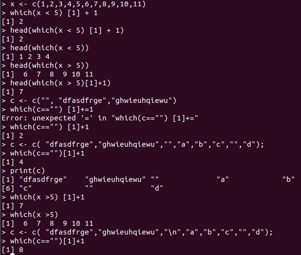
즉 seq함수를 이용해서 text벡터에서 처음으로 공백이 나오는 줄의 다음부터 마지막까지 msg에 저장합니다.
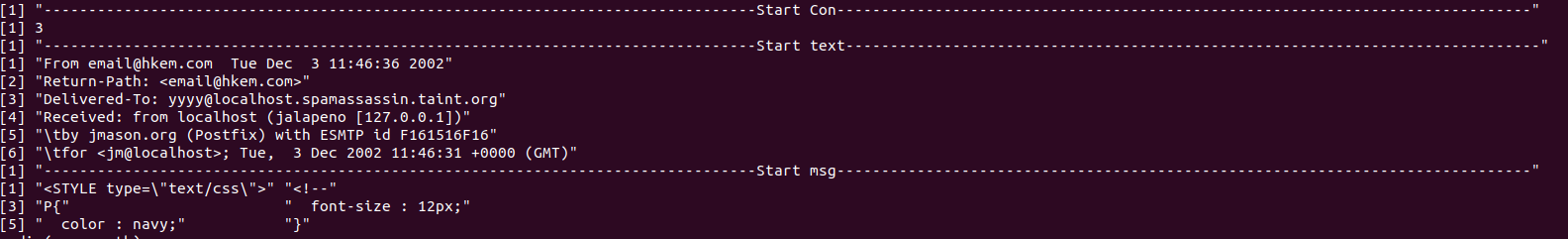
spam.path디렉토리의 모든 파일들을 읽어서 메일의 본문을 all.spam에 벡터형식으로 저장합니다. 그러나 파일중에 cmds파일은 쓸모없는 파일이므로 제외합니다. paste함수를 이용해서 msg객체의 벡터를 한줄로 만듭니다.
spam.docs<-dir(spam.path)
spam.docs<-spam.docs[which(spam.docs!="cmds")]
all.spam<-sapply(spam.docs, function(p) get.msg(paste(spam.path,p,sep="/")))
다음 사진은 실행결과중 일부 입니다.
spam 말뭉치 만들어 내기
 get.tdm<-function(doc.vec){
    doc.corpus<-Corpus(VectorSource(doc.vec))
    control<-list(stopwords=TRUE, removePunctuation=TRUE, removeNumbers=TRUE, minDocFreq=2)
    doc.dtm<-TermDocumentMatrix(doc.corpus,control)
    return(doc.dtm)
 }

spam.tdm<-get.tdm(all.spam)
VectorSource함수는 각 벡터 원소를 하나의 문서로 해석합니다.
Corpus 함수는 문서의 모음(?)으로 만든다고합니다.
get.tdm은 문서의 모음에서 불용어를 제거하고, 구두점도 제거하고, 숫자도 제거하고, 말뭉치에서 한번 이상 나타난 단어들만 용서-문서테이블로 만들어줍니다.
spam 분류기 개발
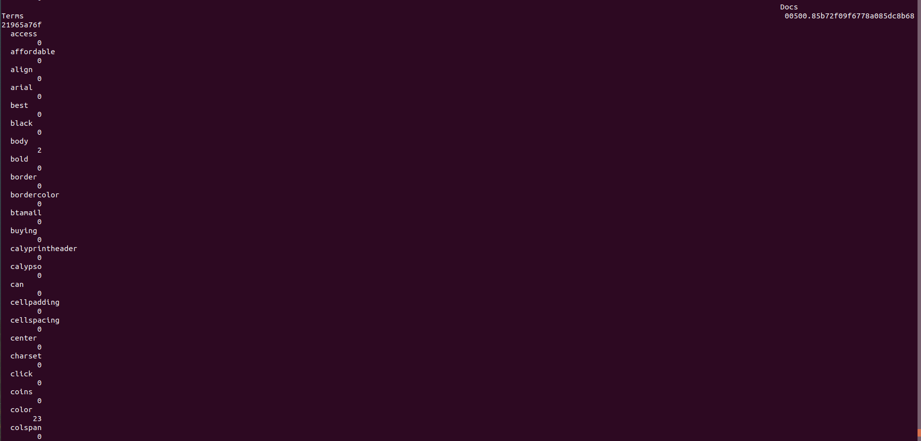
spam.tdm을 표준 R행렬로 변환합니다.
spam.matrix <- as.matrix(spam.tdm)
다음은 spam.matrix의 일부입니다. 행렬의 행은 단어, 열은 문서입니다.
모든 문서의 단어 출현수를 더합니다.
spam.counts<-rowSums(spam.matrix)
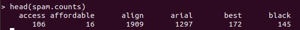
다음은 spam.counts의 일부입니다.
단어열과 출현 빈도수열을 뽑아서 데이터 프레임을 다시 만듭니다.
spam.df<-data.frame(cbind(names(spam.counts),as.numeric(spam.counts)),stringsAsFactors=FALSE)
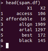
다음은 spam.df의 일부입니다.
spam.df의 각 열에 term, frequency라는 이름을 부여하고 문자형인 frequency열을 숫자형으로 바꿉니다.
names(spam.df)<-c("term", "frequency")
spam.df$frequency<-as.numeric(spam.df$frequency)
주어진 단어가 나타나는 문서의 비율을 계산합니다.
spam.occurrence<-sapply(1:nrow(spam.matrix), function(i){
     length(which(spam.matrix[i,]>0))/ncol(spam.matrix)
})
1:nrow(spam.matrix)는 “단어행의 1행~끝행”을 뜻합니다. length(which(spam.matrix[i,])>0)는 단어가 출현한 문서의 개수를 의미하고 ncol(spam.matrix)는 총 문서의 개수를 의미합니다.
마지막으로 단어의 밀도를 구하고 spam.df데이터프레임에 밀도와 출현정도를 추가합니다.
spam.density<-spam.df$frequency/sum(spam.df$frequency)
spam.df<-transform(spam.df, density=spam.density,occurrence=spam.occurrence)
easy햄 과정은 spam과정을 그대로 따라하면 됩니다.
easyham.docs<-dir(easyham.path)
easyham.docs<-easyham.docs[which(easyham.docs!="cmds")]
all.easyham<-sapply(easyham.docs, function(p) get.msg(paste(easyham.path,p,sep="/")))
easyham.tdm<-get.tdm(all.easyham)
easyham.matrix <- as.matrix(easyham.tdm)
easyham.counts<-rowSums(easyham.matrix)
easyham.df<-data.frame(cbind(names(easyham.counts),as.numeric(easyham.counts)),stringsAsFactors=FALSE)
names(easyham.df)<-c("term", "frequency")
easyham.df$frequency<-as.numeric(easyham.df$frequency)
easyham.occurrence<-sapply(1:nrow(easyham.matrix), function(i){
  length(which(spam.matrix[i,]>0))/ncol(spam.matrix)
})
easyham.density<-easyham.df$frequency/sum(easyham.df$frequency)
easyham.df<-transform(easyham.df, density=easyham.density,occurrence=easyham.occurrence)
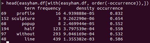
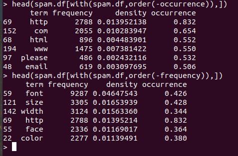
책과는 달리 easyham 단어도 출현 빈도가 높습니다.
분류기로 고난도 햄 검증하기
이메일이 스팸인지 아닌지 검증하려 할때 검증하려는 이메일에 포함된 단어가 학습데이터에 없는 경우가 있습니다. 그런 경우 출현 확률을 0으로 하면 심각한 오류가 생기므로 기본값을 0.0001%로 설정합니다.
 classify.email<-function(path, training.df, prior=0.5, c=1e-6){
    msg<-get.msg(path)
    msg.tdm<-get.tdm(msg)
    msg.freq<-rowSums(as.matrix(msg.tdm))
    msg.match<-intersect(names(msg.freq),training.df$term)
    if(length(msg.match)<1){
       return (prior*c^(length(msg.freq)))
    }
    else{
       match.probs<-training.df$occurrence[match(msg.match, training.df$term)]
       return (prior*prod(match.probs)*c^(length(msg.freq)-length(msg.match)))
    }
 }
분류기 실행해보기
hardham.docs<-dir(hardham.path)
hardham.docs<-hardham.docs[which(hardham.docs!="cmds")]
hardham.spamtest<-sapply(hardham.docs, function(p) classify.email(paste(hardham.path,p,sep="/"),training.df=spam.df))
hardham.hamtest<-sapply(hardham.docs, function(p) classify.email(paste(hardham.path,p,sep="/"),training.df=easyham.df))
hardham.res<-ifelse(hardham.spamtest > hardham.hamtest,TRUE,FALSE)
summary(hardham.res)
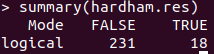
긍정오류율이 18/249 , 7%로 낮습니다.
모든 이메일 종류에 대해 분류기 검증
spam.classifier <-function(path){
pr.spam<-classify.email(path,spam.df)
pr.ham<-classify.email(path, easyham.df)
return(c(pr.spam, pr.ham, ifelse(pr.spam>pr.ham, 1, 0)))
}
easyham2.docs <- dir(easyham2.path)
easyham2.docs <- easyham2.docs[which(easyham2.docs != "cmds")]
hardham2.docs <- dir(hardham2.path)
hardham2.docs <- hardham2.docs[which(hardham2.docs != "cmds")]
spam2.docs <- dir(spam2.path)
spam2.docs <- spam2.docs[which(spam2.docs != "cmds")]
easyham2.class <- suppressWarnings(lapply(easyham2.docs,
function(p)
{
spam.classifier(file.path(easyham2.path, p))
}))
hardham2.class <- suppressWarnings(lapply(hardham2.docs,
function(p)
{
spam.classifier(file.path(hardham2.path, p))
}))
spam2.class <- suppressWarnings(lapply(spam2.docs,
function(p)
{
spam.classifier(file.path(spam2.path, p))
}))
easyham2.matrix <- do.call(rbind, easyham2.class)
easyham2.final <- cbind(easyham2.matrix, "EASYHAM")
hardham2.matrix <- do.call(rbind, hardham2.class)
hardham2.final <- cbind(hardham2.matrix, "HARDHAM")
spam2.matrix <- do.call(rbind, spam2.class)
spam2.final <- cbind(spam2.matrix, "SPAM")
class.matrix <- rbind(easyham2.final, hardham2.final, spam2.final)
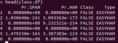
class.df <- data.frame(class.matrix, stringsAsFactors = FALSE)
names(class.df) <- c("Pr.SPAM" ,"Pr.HAM", "Class", "Type")
class.df$Pr.SPAM <- as.numeric(class.df$Pr.SPAM)
class.df$Pr.HAM <- as.numeric(class.df$Pr.HAM)
class.df$Class <- as.logical(as.numeric(class.df$Class))
class.df$Type <- as.factor(class.df$Type)
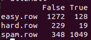
이메일 종류별 긍정오류, 부정오류 계산하기
저난도 햄의 부정오류개수를 구합니다.
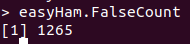
easyHam.False<-subset(class.df, Type=="EASYHAM" & Class=="FALSE")
easyHam.FalseCount<-nrow(easyHam.False)
저난도 햄의 긍정오류개수를 구합니다.
easyHam.True<-subset(class.df, Type=="EASYHAM" & Class=="TRUE")
easyHam.TrueCount<-nrow(easyHam.True)
고난도 햄과 스팸까지 모두 구한후 하나의 데이터 프레임으로 만들면 된다.
easy.row <- c(easyHam.FalseCount, easyHam.TrueCount)
hard.row<-c(HardHam.FalseCount, HardHam.TrueCount)
spam.row<-c(spam.FalseCount, spam.TrueCount)
allEmail<-rbind(easy.row, hard.row,spam.row)
colnames(allEmail) = c("False", "True")
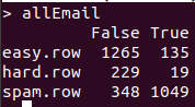
분류결과가 좋습니다. 그러나 책과는 다르게 긍정오류율보다 부정오류율이 더 높습니다.
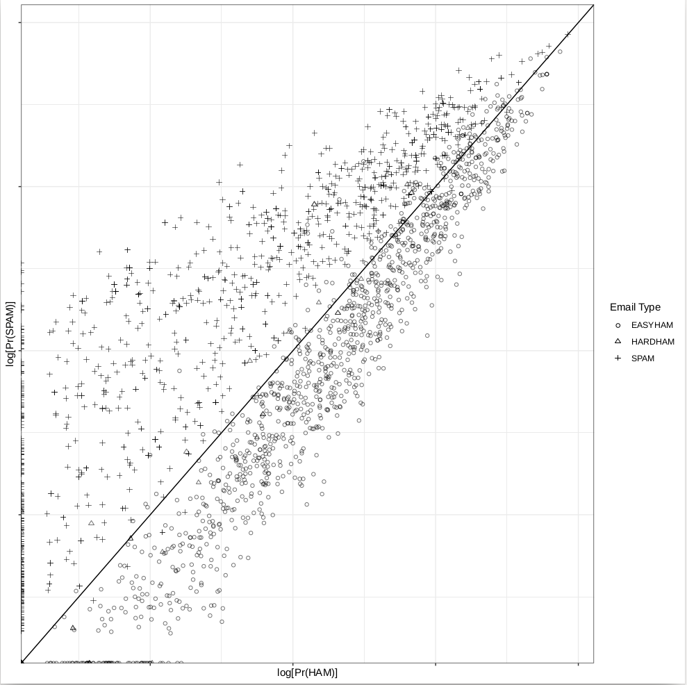
그래프
class.plot <- ggplot(class.df, aes(x = log(Pr.HAM), log(Pr.SPAM))) +
    geom_point(aes(shape = Type, alpha = 0.5)) +
    geom_abline(intercept = 0, slope = 1) +
    scale_shape_manual(values = c("EASYHAM" = 1,
                                  "HARDHAM" = 2,
                                  "SPAM" = 3),
                       name = "Email Type") +
    scale_alpha(guide = "none") +
    xlab("log[Pr(HAM)]") +
    ylab("log[Pr(SPAM)]") +
    theme_bw() +
    theme(axis.text.x = element_blank(), axis.text.y = element_blank())
ggsave(plot = class.plot,
       filename = file.path("./", "03_final_classification.pdf"),
       height = 10,
       width = 10)
get.results <- function(bool.vector)
{
         results <- c(length(bool.vector[which(bool.vector == FALSE)]) / length(bool.vector),
              length(bool.vector[which(bool.vector == TRUE)]) / length(bool.vector))
 return(results)
}
stat_abline은 ggplot2라이브러리에서 삭제된 함수입니다. 대신에 geom_abline을 사용합니다.
결과개선
실제 햄대 스팸 비율이 80대 20인 사실을 바탕으로 함수를 수정합니다.
spam.classifier <-function(path){
  pr.spam<-classify.email(path,spam.df, prior=0.2)
  pr.ham<-classify.email(path, easyham.df, prior=0.8)
  return(c(pr.spam, pr.ham, ifelse(pr.spam>pr.ham, 1, 0)))
}
##부정, 긍정오류 결과
easyham2.col <- get.results(subset(class.df, Type == "EASYHAM")$Class)
hardham2.col <- get.results(subset(class.df, Type == "HARDHAM")$Class)
spam2.col <- get.results(subset(class.df, Type == "SPAM")$Class)

class.res <- rbind(easyham2.col, hardham2.col, spam2.col)
colnames(class.res) <- c("NOT SPAM", "SPAM")
print(class.res)
전
후
이지햄 결과가 조금 다른것 말고 큰차이가 없습니다.
그래프
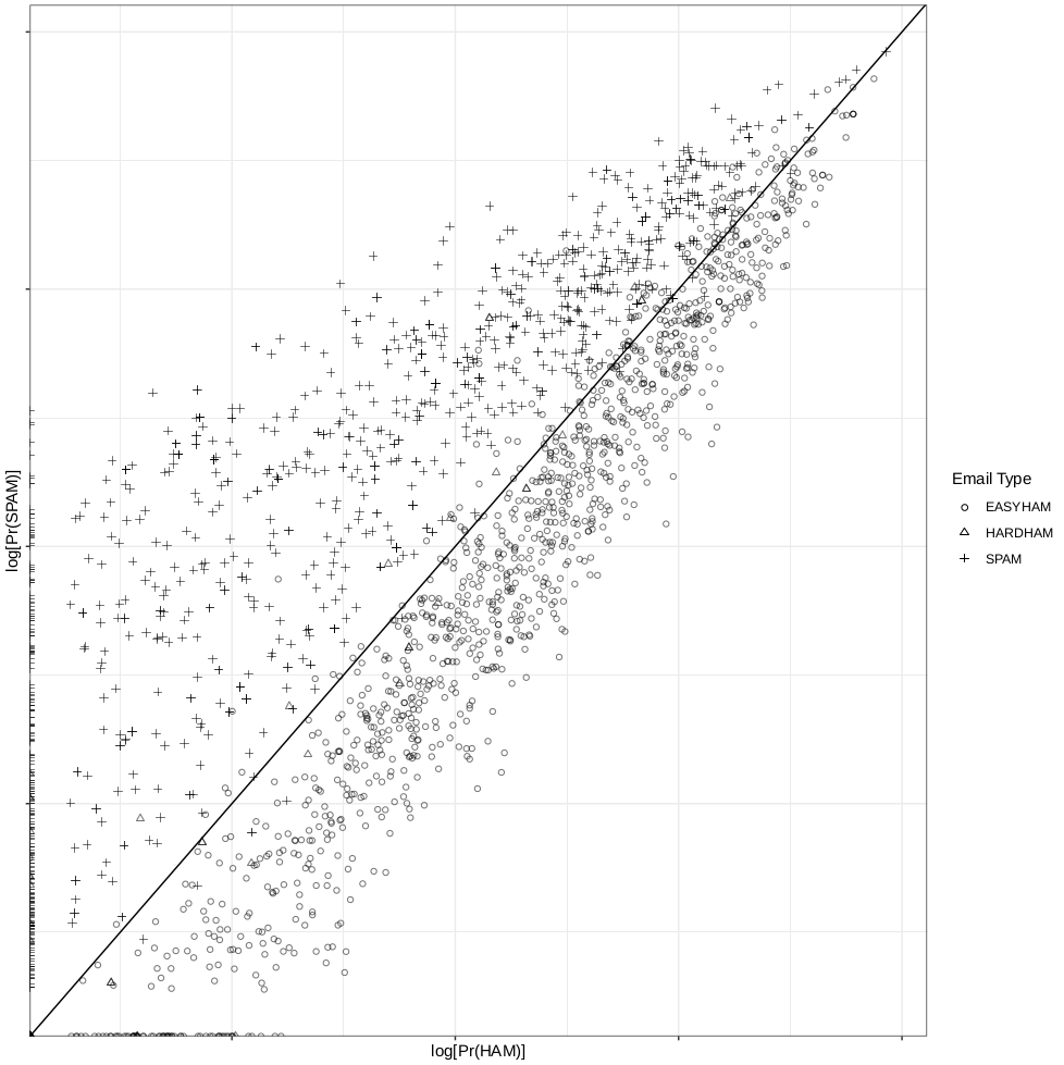 그래프도 큰차이가 없습니다.
** 모든 내용은 강릉원주대학교 강태원 교수님의 ‘데이터 마이닝’강의와 드류 콘웨이 와 존 마일스 화이트의’해커스타일로 배우는 기계학습’를 토대로 작성했습니다.**
Machine Learning for Hackers License
All source code is copyright (c) 2012, under the Simplified BSD License. For more information on FreeBSD see: http://www.opensource.org/licenses/bsd-license.php
All images and materials produced by this code are licensed under the Creative Commons Attribution-Share Alike 3.0 United States License: http://creativecommons.org/licenses/by-sa/3.0/us/